படிமம்:Airflow-Obstructed-Duct.png
Jump to navigation
Jump to search
இந்த முன்னோட்டத்தின் அளவு: 800 × 571 படப்புள்ளிகள் . மற்ற பிரிதிறன்கள்: 320 × 229 படப்புள்ளிகள் | 640 × 457 படப்புள்ளிகள் | 1,024 × 731 படப்புள்ளிகள் | 1,270 × 907 படப்புள்ளிகள் .
மூலக்கோப்பு (1,270 × 907 படவணுக்கள், கோப்பின் அளவு: 85 KB, MIME வகை: image/png)
சுருக்கம்

|
File:N S Laminar.svg என்பது இந்தக் கோப்பின் திசையன் வடிவமாகும். இந்தக் PNG கோப்பின் இடத்தில் திசையன் கோப்புத் தரம் குறைவாக இல்லாவனில் இதைப் பயன்படுத்த வேண்டும்.
File:Airflow-Obstructed-Duct.png → File:N S Laminar.svg
மேலும் தகவலுக்கு, உதவி:SVG பார்க்கவும். |
 |
| விளக்கம் |
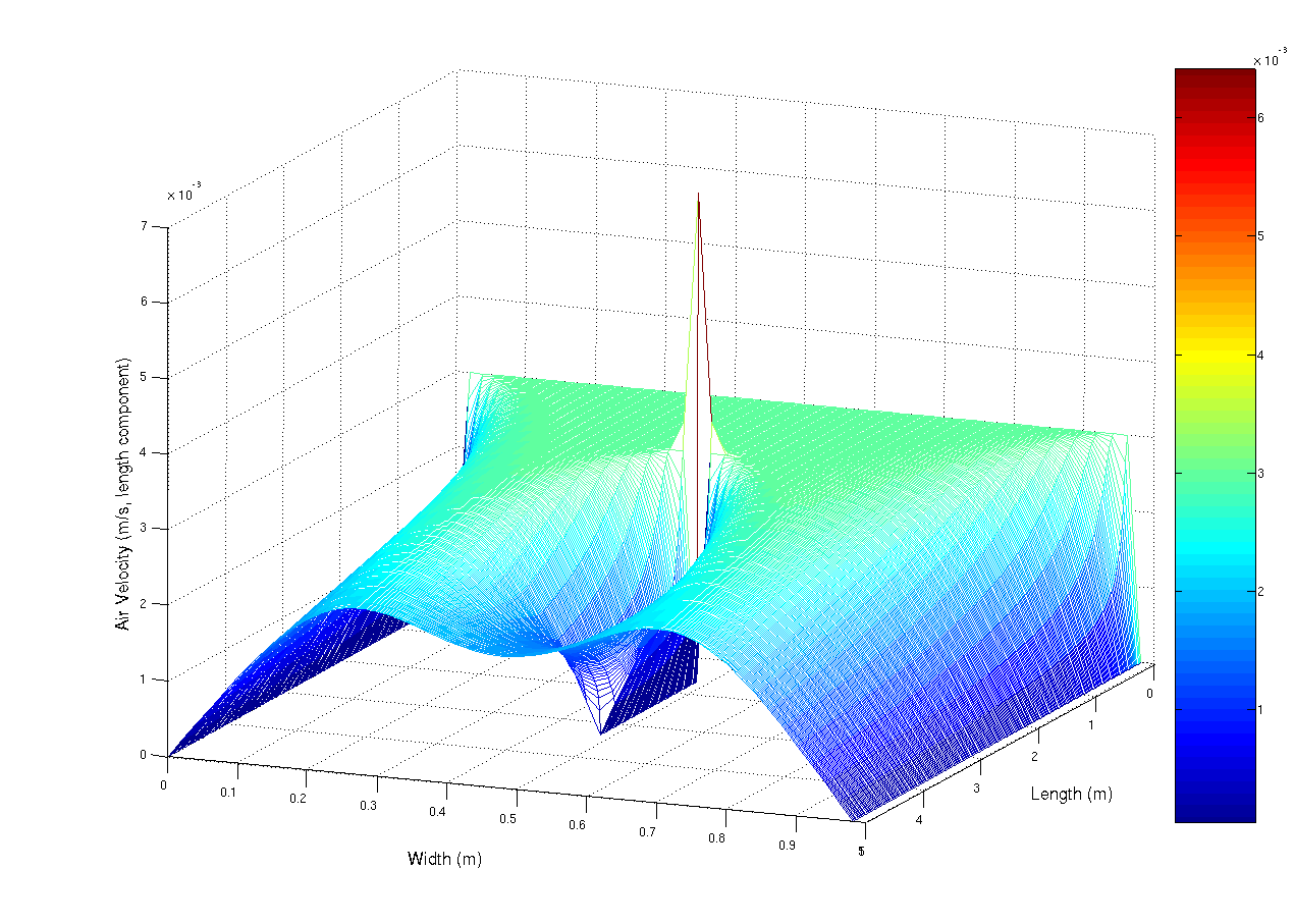
A simulation using the navier-stokes differential equations of the aiflow into a duct at 0.003 m/s (laminar flow). The duct has a small obstruction in the centre that is parallel with the duct walls. The observed spike is mainly due to numerical limitations. This script, which i originally wrote for scilab, but ported to matlab (porting is really really easy, mainly convert comments % -> // and change the fprintf and input statements) Matlab was used to generate the image.
%Matlab script to solve a laminar flow
%in a duct problem

%Constants
inVel = 0.003; % Inlet Velocity (m/s)
fluidVisc = 1e-5; % Fluid's Viscoisity (Pa.s)
fluidDen = 1.3; %Fluid's Density (kg/m^3)

MAX_RESID = 1e-5; %uhh. residual units, yeah...
deltaTime = 1.5; %seconds?
%Kinematic Viscosity
fluidKinVisc = fluidVisc/fluidDen;

%Problem dimensions
ductLen=5; %m
ductWidth=1; %m

%grid resolution
gridPerLen = 50; % m^(-1)
gridDelta = 1/gridPerLen;
XVec = 0:gridDelta:ductLen-gridDelta;
YVec = 0:gridDelta:ductWidth-gridDelta;

%Solution grid counts
gridXSize = ductLen*gridPerLen;
gridYSize = ductWidth*gridPerLen;

%Lay grid out with Y increasing down rows
%x decreasing down cols
%so subscripting becomes (y,x) (sorry)
velX= zeros(gridYSize,gridXSize);
velY= zeros(gridYSize,gridXSize);
newVelX= zeros(gridYSize,gridXSize);
newVelY= zeros(gridYSize,gridXSize);

%Set initial condition

for i =2:gridXSize-1
for j =2:gridYSize-1
velY(j,i)=0;
velX(j,i)=inVel;
end
end

%Set boundary condition on inlet
for i=2:gridYSize-1
velX(i,1)=inVel;
end

disp(velY(2:gridYSize-1,1));

%Arbitrarily set residual to prevent
%early loop termination
resid=1+MAX_RESID;

simTime=0;

while(deltaTime)
 count=0;
while(resid > MAX_RESID && count < 1e2)
 count = count +1;
for i=2:gridXSize-1
for j=2:gridYSize-1
newVelX(j,i) = velX(j,i) + deltaTime*( fluidKinVisc / (gridDelta.^2) * ...
(velX(j,i+1) + velX(j+1,i) - 4*velX(j,i) + velX(j-1,i) + ...
velX(j,i-1)) - 1/(2*gridDelta) *( velX(j,i) *(velX(j,i+1) - ...
velX(j,i-1)) + velY(j,i)*( velX(j+1,i) - velX(j,i+1))));

newVelY(j,i) = velY(j,i) + deltaTime*( fluidKinVisc / (gridDelta.^2) * ...
(velY(j,i+1) + velY(j+1,i) - 4*velY(j,i) + velY(j-1,i) + ...
velY(j,i-1)) - 1/(2*gridDelta) *( velY(j,i) *(velY(j,i+1) - ...
velY(j,i-1)) + velY(j,i)*( velY(j+1,i) - velY(j,i+1))));
end
end

%Copy the data into the front
for i=2:gridXSize - 1
for j = 2:gridYSize-1
velX(j,i) = newVelX(j,i);
velY(j,i) = newVelY(j,i);
end
end

%Set free boundary condition on inlet (dv_x/dx) = dv_y/dx = 0
for i=1:gridYSize
velX(i,gridXSize)=velX(i,gridXSize-1);
velY(i,gridXSize)=velY(i,gridXSize-1);

    end

    %y velocity generating vent
    for i=floor(2/6*gridXSize):floor(4/6*gridXSize)
        velX(floor(gridYSize/2),i) = 0;
        velY(floor(gridYSize/2),i-1) = 0;
    end

%calculate residual for
%conservation of mass
resid=0;
for i=2:gridXSize-1
for j=2:gridYSize-1
%mass continuity equation using central difference
%approx to differential
resid = resid + (velX(j,i+ 1)+velY(j+1,i) - ...
(velX(j,i-1) + velX(j-1,i)))^2;
end
end

resid = resid/(4*(gridDelta.^2))*1/(gridXSize*gridYSize);
fprintf('Time %5.3f \t log10Resid : %5.3f\n',simTime,log10(resid));


simTime = simTime + deltaTime;
end
mesh(XVec,YVec,velX)
deltaTime = input('\nnew delta time:');
end
%Plot the results
mesh(XVec,YVec,velX)
|
| நாள் | 24 பெப்ரவரி 2007 (original upload date) |
| மூலம் | Transferred from en.wikipedia to Commons. |
| ஆசிரியர் | User A1 at ஆங்கிலம் விக்கிப்பீடியா |
அனுமதி
| This work has been released into the public domain by its author, User A1 at ஆங்கிலம் விக்கிப்பீடியா. This applies worldwide. சில நாடுகளில் இது சாத்தியமில்லாது போகலாம். அவ்வாறாயின் : User A1 grants anyone the right to use this work for any purpose, without any conditions, unless such conditions are required by law. |
Original upload log
The original description page was here. All following user names refer to en.wikipedia.
- 2007-02-24 05:45 User A1 1270×907×8 (86796 bytes) A simulation using the navier-stokes differential equations of the aiflow into a duct at 0.003 m/s (laminar flow). The duct has a small obstruction in the centre that is paralell with the duct walls. The observed spike is mainly due to numerical limitatio
கோப்பின் வரலாறு
குறித்த நேரத்தில் இருந்த படிமத்தைப் பார்க்க அந்நேரத்தின் மீது சொடுக்கவும்.
| நாள்/நேரம் | நகம் அளவு சிறுபடம் | அளவுகள் | பயனர் | கருத்து | |
|---|---|---|---|---|---|
| தற்போதைய | 16:52, 1 மே 2007 | | 1,270 × 907 (85 KB) | wikimediacommons>Smeira | {{Information |Description=A simulation using the navier-stokes differential equations of the aiflow into a duct at 0.003 m/s (laminar flow). The duct has a small obstruction in the centre that is paralell with the duct walls. The observed spike is mainly |
கோப்பு பயன்பாடு
பின்வரும் பக்க இணைப்புகள் இப் படிமத்துக்கு இணைக்கபட்டுள்ளது(ளன):